Cédric Beaume

Applied Mathematician

You are in Research > Spatial localization

Spatial localization

Spatially localized solutions are a class of physical solutions displaying different states at different spatial locations. They are found in a broad range of systems including fluids (cf coupled convection), buckling problems, chemical reactions and optics. Despite the fundamental difference in the nature of these systems, spatial localization often exhibits similar features. In particular, the stationary localized states lie on branches having a similar structure in parameter space. They are usually compared to results of the simpler Swift–Hohenberg equation which has now become a paradigm for the study of localized states. Two main types of localized states have been observed depending on whether they involve a patterned state or not. The former case yields a behavior called snaking while the latter produces a branch whose solutions grow in energy at a fixed value of the parameter. Both these behaviors underlie the fact that there exists a large number of solutions at specific values of the parameter. Some localized solutions have been found to play an important role in the dynamics of physical systems by either being stable, by attracting transients along their stable manifold or by corresponding to minimal seeds to trigger an instability.

Snaking localized states

Snaking states are observed when fronts pin a spatially periodic state to some other state (for instance, a homogeneous background). Because one of the states is spatially periodic, the fronts are locked at a specific phase along the pattern and cannot move freely. The branches bearing such localized states describe oscillations in parameter space around the Maxwell point where the two states involved have the same value of a free energy. During each oscillation along the snaking, the patterned structure grows spatially by adding one period of the pattern. This behavior is called homoclinic snaking as it concerns homoclinic orbits in space and by analogy to the zig-zags snakes display. For a given problem, different parity solutions may exist yielding intertwined branches of localized solutions (figure 1).

Nonsnaking localized states

When the spatially localized solutions consist of fronts connecting two homogeneous states, snaking is not observed. In that case, the solution has no phase and the fronts can be moved freely at the Maxwell point between both homogeneous states without changing the free energy of the solution. This results in the existence of a continuum of localized solutions at the Maxwell point, each differing only by the location of the fronts. In the usual representation "norm vs parameter", the branch bearing these solutions would display a vertical growth located at the Maxwell point between the two states involved (figure 2).

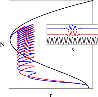Figure 1: Norm N of solutions from the quadratic-cubic Swift–Hohenberg equation versus the forcing parameter r. The inset represents one solution along each branch. In black: periodic states. In red and blue are represented the different parity localized states. Dashed line: Maxwell point between the trivial solution (bottom axis) and the periodic states.

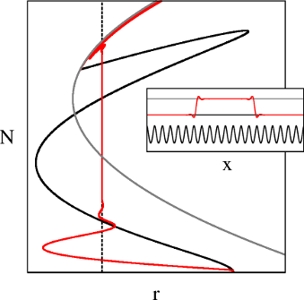Figure 2: Same as figure 1 but for different parameters. In black: periodic states. In red: localized states consisting in fronts connecting the trivial state (black in the inset, bottom axis in the bifurcation diagram) to the other homogeneous one (grey). Dashed line: Maxwell point between the trivial state and the homogeneous one.

© ~ 2011–2020 ~ Cédric Beaume